
This article explains how to use Aura's Change Detection and Convergence Monitoring workflow to compare two Hovermap scans of the same area and visualize changes between them. The result is a point cloud with point-to-mesh distance attributes and a mesh file generated from the reference scan.
Aura's Change Detection and Convergence Monitoring solution integrates the rapid data capture capabilities of Hovermap with Aura's processing and analysis to help manage and monitor excavation projects. Tailored for underground environments and enclosed spaces, the solution captures current excavation profiles with Hovermap, then processes, aligns, and visualizes changes in Aura.
The following video shows how to use Aura to compare two Hovermap scans of the same area.
What you will need
Operating system: Windows 10
Aura: Version 1.8.1 or higher
Entitlement: A valid SLAM and Convergence Monitoring license
Point cloud data: 2 Hovermap scans of the same area, with the original .bag files for both scans
This solution is designed and optimized for use in underground mining (drives and tunnels) and other internal enclosed spaces. It may not be suitable for other environments.
Scans can be captured by walking, driving, or flying.
Before running the Convergence Monitoring workflow, both scans must be processed using SLAM.
How it works
The basic process for change detection and convergence monitoring involves taking the reference scan, creating a mesh of that reference scan, and then measuring the distance from the points in the second scan (of the same area) to the mesh.
.png)
Procedure
Step 1: Configure the convergence monitoring job
Open Aura. Ensure an active SLAM and Convergence monitoring license is present.
In the Process tab, click Process Scan.
In the Configure New Scan Job panel, select the Convergence monitoring workflow.
Click Add Datasets.
In the dialog box that displays, click Add, then browse for the point clouds to use.
Ensure the point clouds have been pre-processed in the latest version of Aura.
In the Alignment Preview File column, select the scan file to use for alignment.
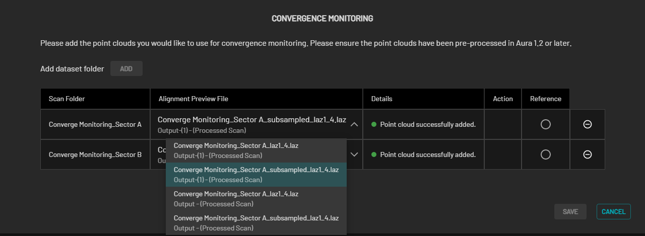
Convergence Monitoring is performed on the full point cloud regardless of the selected Alignment Preview File. Use only the subsampled files to lower the computational resources needed, especially for large datasets. The reduced set of points on a subsampled file also helps focus on key features for more accurate alignment.
Select the reference scan file. The reference scan provides a fixed frame of reference for aligning the other point cloud, establishing a coordinate system that other scans can be transformed into.
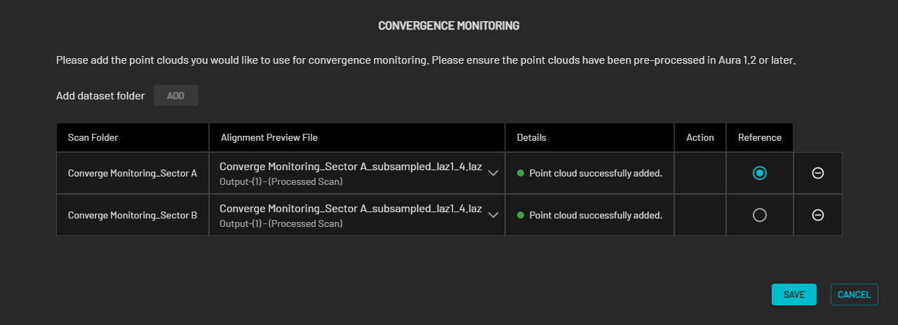
Once the point clouds have been added and the reference scan selected, click Save.
In the Location field, enter the preferred name for the output folder and select the output folder location.
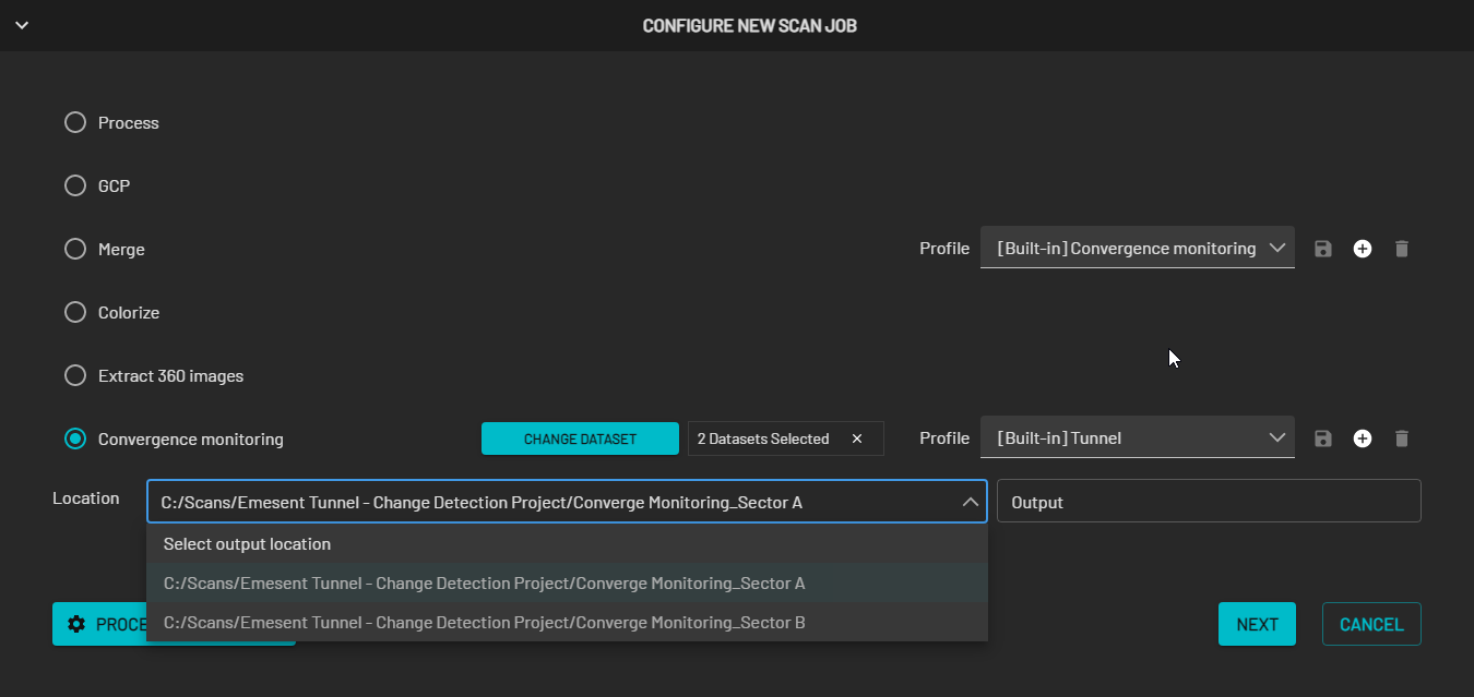
Select the profile to use.
.png)
Click Processing Settings to configure the convergence parameters. See the Processing settings section below for detailed information.
Skip this step to process using the default settings.
Click Next.
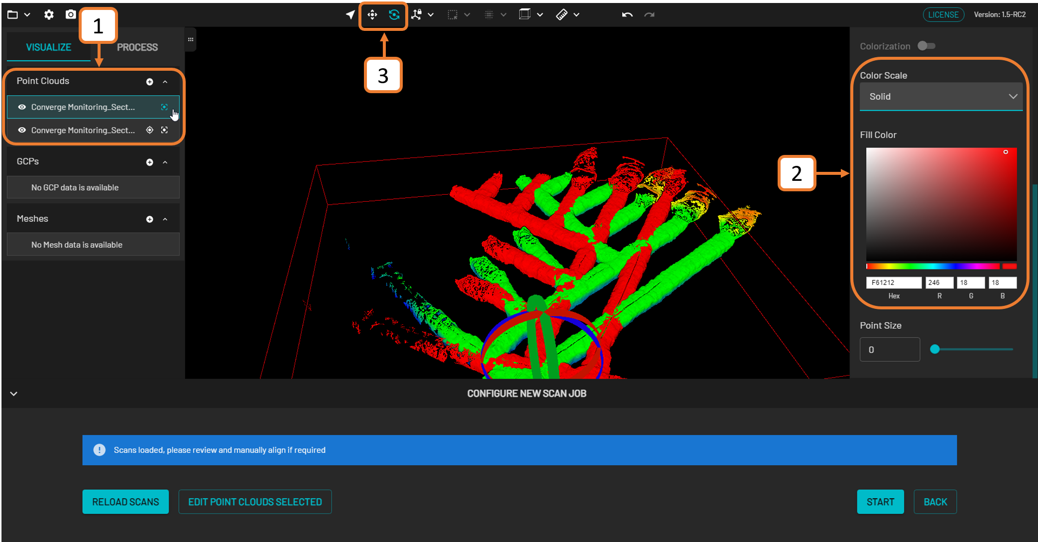
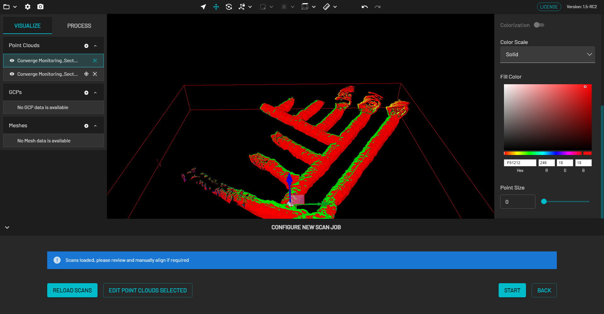
Step 2: Review and manually align the datasets
Click Load Scans to start the review. All scans load at the same time.
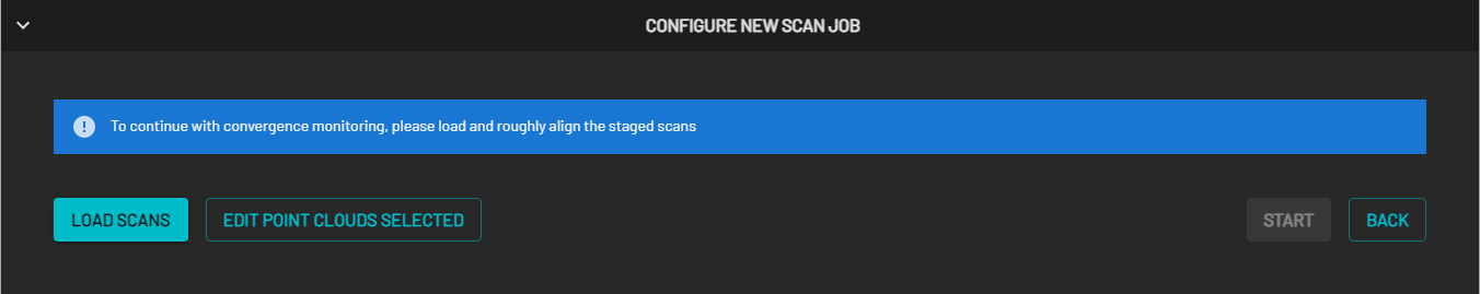
If the incorrect dataset was selected, click Edit Point Clouds Selected to load the correct ones.
Follow these guidelines to roughly align the second scan with the reference scan:
Ensure the second scan is selected in the Visualize tab under the Point Clouds menu.
Use the Transform and Rotate tools to align the point clouds.
When using the Rotate tool, the following shortcut keys change the pivot point of the rotation:
CTRL+Shift+C: Changes the origin point to the newly selected point. Click an area on the second scan to select a new origin point.
Ctrl+Shift+Z: Resets the origin point back to the point cloud's origin.
Once the scans have been roughly aligned, click Start.
Step 3: Start processing
After clicking Start, a progress bar shows how far along the processing job is. The elapsed time of the processing job is shown to the right.
The directory file path below the progress bar provides a way to identify the dataset source. This is useful if multiple jobs are processed simultaneously with the same output folder name. Copying the file path and pasting it into the file explorer allows access to the completed files without waiting for the processing job to be completed.
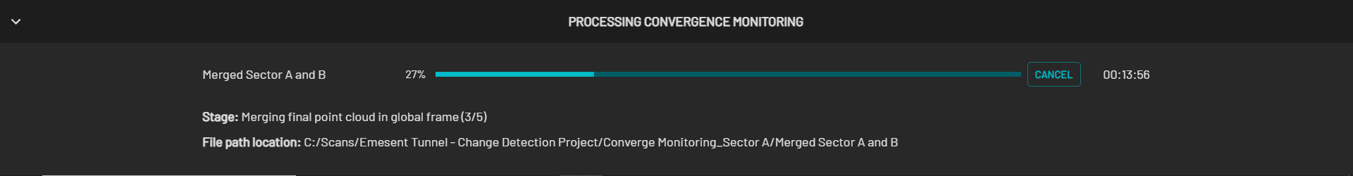
The Retry button becomes available when a failure occurs during processing. Click to attempt to process the current job from the last successful stage.
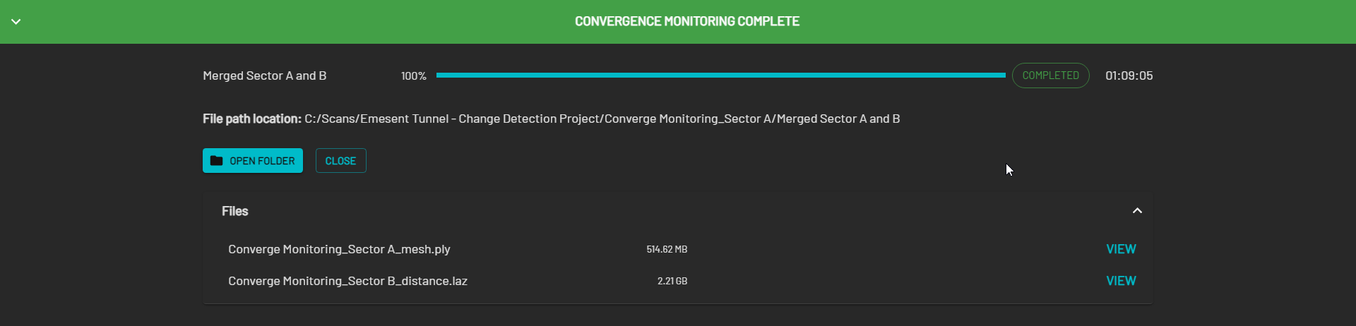
Step 4: Inspect the final output
Once processing is complete, two output files are generated:
Output | Description |
|---|---|
.LAZ | Point cloud with point-to-mesh distance attributes. |
.PLY | Mesh file created from the reference scan. |
Click View to display the generated .LAZ file in the Viewport.
Currently, aside from viewing the .PLY file, there are no options to interact with a Mesh file.
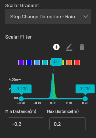
In the Context Panel on the right, click Color Scale, then select Distance from the drop-down menu. The Step Change Detection - Rainbow color gradient is automatically selected.
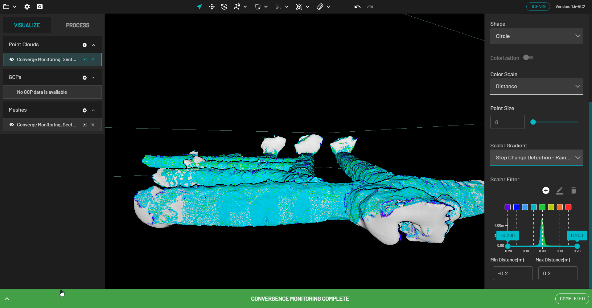
The colors and distance values can be edited within the Scalar Filter. The distance points included in the final output file (.LAZ) can also be adjusted:
ADD: Click the + icon, then select a color and specify the Location in meters.
EDIT: Click the square color box, then click the Pencil icon.
DELETE: Click the square color box, then click the Trash icon.
Use the near clip plane (by holding the ALT key while using the mouse scroll wheel in Perspective mode) to view and navigate inside the tunnel.
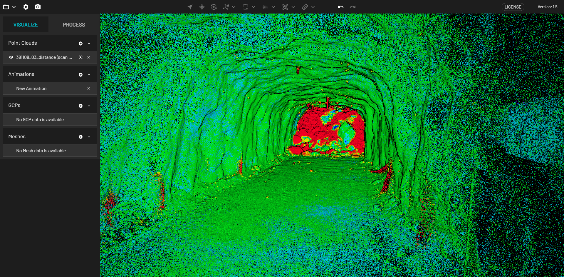
Pieces of infrastructure (such as pipes, rock bolts, fans) may show changes due to how the meshing process removes and smooths out those features on the reference scan. These changes can typically be ignored.
Outcome
The two scans have been processed and aligned, and the resulting .LAZ point cloud is available for viewing with point-to-mesh distance attributes color-coded by the Step Change Detection - Rainbow gradient. The corresponding .PLY mesh file generated from the reference scan is also available in the output folder.
Additional information
Processing settings
Alignment settings can be changed via the Merge and Meshes tabs in Processing Settings.
When the settings on a built-in processing profile are updated in Aura, a temporary Custom profile is created, which can be used in any of the workflows for the current session. Save this custom profile to save time setting up processing jobs for common or known environments. Once saved, it becomes available for selection in the Profiles dropdown list.
Custom profiles that are not saved are automatically removed when the application is closed.
Merge tab
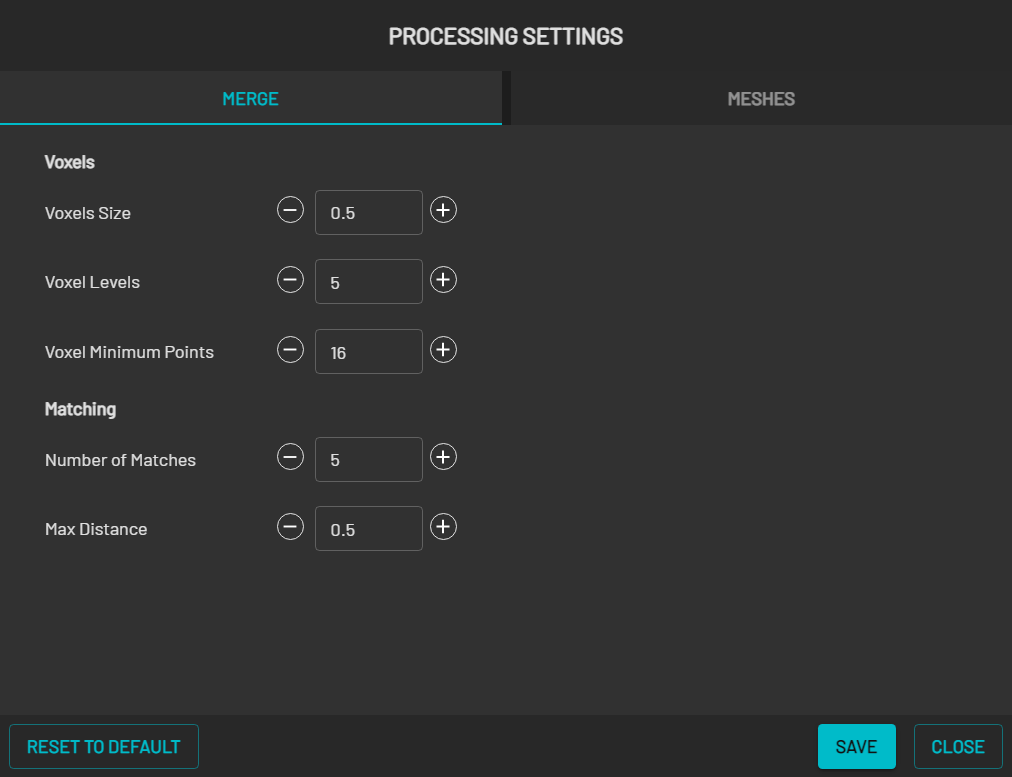
Field | Description |
|---|---|
Voxels |
|
Matching |
|
Meshes tab
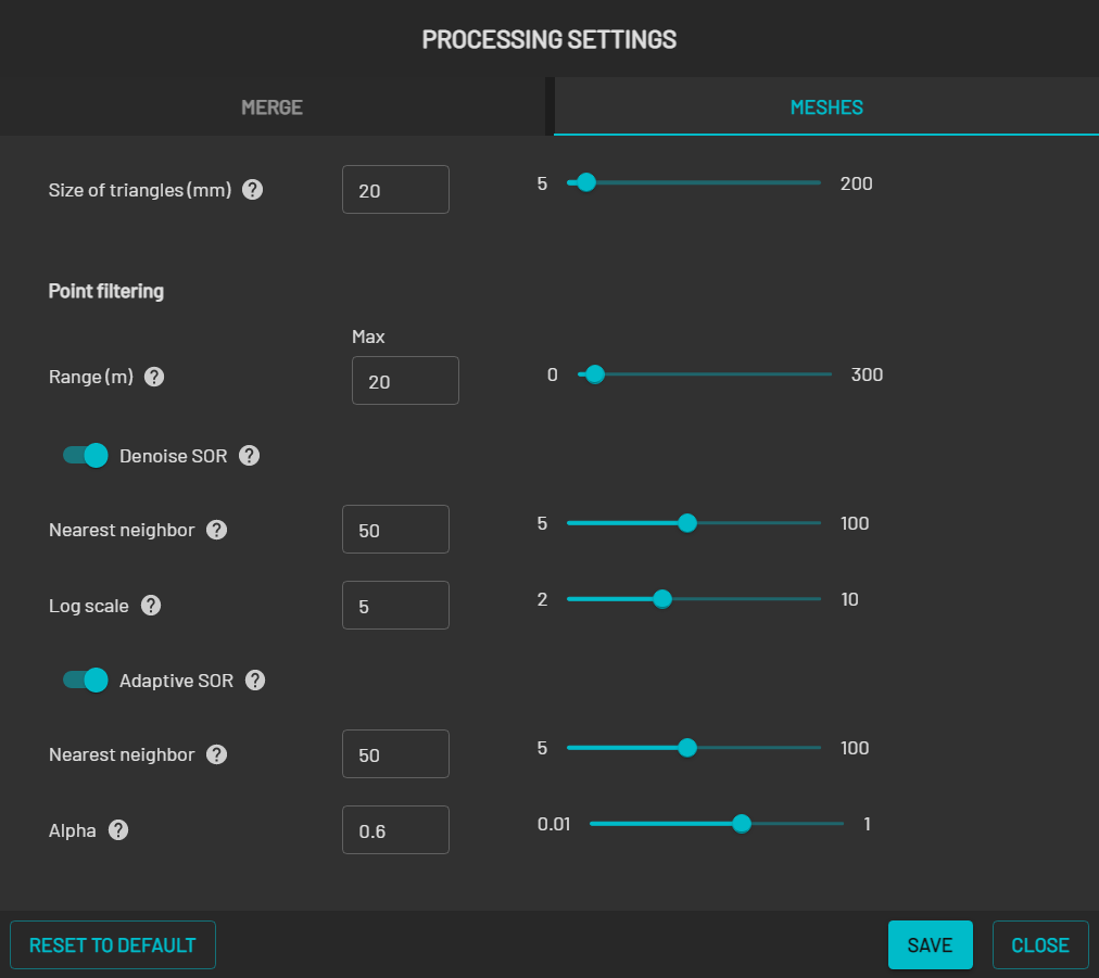
Field | Description |
|---|---|
Size of triangles (mm) | The level of detail that makes up the 3D mesh. A smaller triangle size results in a more detailed mesh. |
Point filtering (m) |
|